ML from Scratch Episode 1: Math Behind Machine Learning and Gradient Descent Algorithm

I got the greatest opportunity to revisit ML once again from scratch, and I want to utilize this chance to do it right. I want to begin this journey at the right place, and that would be the “Foundations—the Math behind Machine Learning.” Most learners are reluctant to step into this zone, not because it is difficult, but because of an uncomfortable lie we spread amongst ourselves: ML Math is hard. But well to be honest, it ain’t easy and I won’t deny that, but it is also a straightforward truth that it is not impossible. With the right material and the right tutorial, even the math behind ML can become a comfortable concept. In this blog post, I aim to outline the necessary math concepts that serve as prerequisites for ML. I will give a very generic introduction, but the deep dive and practice are something I leave up to you.

Math Concepts that are prerequisites of ML

Calculus

Calculus was one of the scariest math concepts to me growing up. Truth be told, I am still a little intimidated by its profundity and complexity. But that is also the most exciting part that allured me towards it. Calculus plays a very primal role in the gradient descent algorithm, which is literally the backbone of almost every ML algorithm that exists today. And with that level of prominence, it is only natural to start with this topic first.

Derivatives and Partial Derivatives:

A very formal definition of a derivative is the instantaneous rate of change. Consider a car moving through distance s in time t. The rate of change of speed (or velocity, if in a particular direction) is the rate at which the car covers distance per unit change in time. Let’s denote this as:

v (speed/velocity) = change in distance / change in time

Now, what is d/dt (s)? It is essentially calculating the instantaneous rate of change in distance with respect to the change in time, represented by dt.

Here is where it gets tricky: as the unit time approaches 0, the change in distance approaches a constant. Tricky? Let me explain. A car speeding down a road is constantly being measured with respect to time—per unit time, how much distance is it covering precisely? But as we freeze time, the distance covered becomes a snapshot of the car at one particular instance. At that frame, the car’s speed is no longer a variable but a fixed constant value obtained at that specific snapshot.

Okay, before you get bored, here is what I am trying to infer from this example: the rate of change of distance with respect to time—aka the speed—is a variable. Now when I apply a derivative to it, I am getting the instantaneous rate of change at a particular instant, and my speed becomes a constant.

A better definition of a derivative would be—the best constant approximation of the rate of change.

Sound familiar? I just applied d/dx (x) and my result is a constant. The old school math taught us that d/dx (x) is a constant, but we never fully grasped why.

Derivatives give a lot of insight into functions, and in ML, we deal with functions everywhere. Every ML algorithm revolves around an objective function that needs to be optimized, and gradient descent is essentially finding the minimum of the cost function by leveraging derivatives.

Here are a few derivative concepts one should know to understand gradient descent algorithm:

• Sum Rule: The derivative of a sum is the sum of the derivatives. Simple, yet foundational when dealing with multiple loss terms.
• Product Rule: When you have a product of two functions, f(x) and g(x), the derivative is f'(x)g(x) + f(x)g'(x).
• Chain Rule: This is the heavy lifter. If you have a composite function f(g(x)), its derivative is f'(g(x)) * g'(x). In deep learning, this is what enables backpropagation—the chain rule allows us to propagate errors backward through layers of a neural network.

Gradient: A formal deifinition of a gradient would be the vector of all partial derivatives of a function. Points in the direction of steepest ascent. We will explore gradient descent algorithm a little later in this article, but just to give the context, a gradient would be a derivate of a function w.r.t multivariables (please refer to multivariate calculus and vector calculus for more info) aka the trainable paramaters. A general rule of thumb is that, Gradient descent moves in the opposite direction of the gradient to minimize loss: θ = θ - α∇L(θ), where α is learning rate. Learning rate is a hyperparameter that decides the training process. Too high means too much divergence from the required objective and too low means painfully slow training.

Jacobian and Hessian Matrices:

Jacobian is a matrix of all first-order partial derivatives when you have multiple outputs and multiple inputs (a function f: Rⁿ → Rᵐ). Each row is the gradient of one output w.r.t. all inputs. Used in backprop when passing gradients through layers with vector outputs. Hessian is a matrix of all second-order partial derivatives — tells you about curvature of the loss surface. Used conceptually in second-order optimization methods (Newton’s method) and to distinguish minima/maxima/saddle points (via eigenvalues of the Hessian — positive definite = local min).

Linear Algebra

If Calculus is the engine, Linear Algebra is the vehicle. While calculus helps us understand how to change, linear algebra gives us the structural framework to handle large-scale, multi-dimensional data. In simpler terms, if your ML algorithm is a dish, Calculus is the recipe, whereas Linear Algebra is the bowl and probability is the measure of ingredients.

In ML, almost all data is represented as vectors or matrices. A single feature set is a vector; a whole dataset is a matrix. When we talk about a model “learning,” we are essentially talking about performing transformations on these matrices.

Vectors and Matrices:

Think of a dataset with n features as a point in an n-dimensional space. Matrix multiplication allows us to transform this point from the input space to a different output space. It clicked for me when I realized that a simple linear regression, y = Wx + b, is not just an equation—it is a geometric transformation of the input vector x using the weight matrix W and a bias shift b.

Dot Products:

The dot product measures similarity or alignment between two vectors. In a neural network, each neuron essentially computes a dot product between the input vector and its weight vector.

Eigenvalues and Eigenvectors:

While you don’t need these on day one, they are crucial for dimensionality reduction techniques like PCA (Principal Component Analysis), which help us compress data without losing too much information.

Eigenvector: a vector that doesn’t change direction when a matrix transformation is applied to it — only gets scaled. Eigenvalue: the scale factor.

PCA (Principal Component Analysis) finds the eigenvectors of the covariance matrix of your data — these are the directions of maximum variance. This is literally how dimensionality reduction works.

Understanding Linear Algebra shifts your perspective from “numbers in tables” to “objects moving in space.” It makes the abstract nature of high-dimensional data surprisingly tangible.

Probability

Machine Learning is fundamentally about dealing with uncertainty. Our data is noisy; our samples are finite; the real world is stochastic. Probability provides the mathematical language to describe this uncertainty.

• Random Variables and Distributions: We assume our data is generated from some underlying probability distribution (often Gaussian). The goal of ML is to estimate the parameters of this distribution so we can predict the likelihood of new data points.
• Maximum Likelihood Estimation (MLE): This is a profound bridge between statistics and ML. MLE states that we should choose model parameters that maximize the probability (likelihood) of observing our training data. Guess what? Many common loss functions are direct results of MLE. For instance, minimizing the Mean Squared Error (MSE) is mathematically equivalent to maximizing the likelihood under a Gaussian noise assumption.
• Bayes’ Theorem: This allows us to update our beliefs based on new evidence. It forms the backbone of Bayesian Machine Learning and is crucial for concepts like Naive Bayes classifiers.

Probability gives us the justification for why we choose specific loss functions and why we expect our models to generalize to unseen data.

Gradient Descent: The Unifying Algorithm

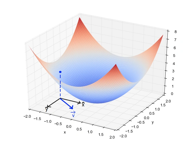
Now, let’s connect all the dots. We have the objective (Probability/Cost function), the high-dimensional space (Linear Algebra), and the tool for movement (Calculus). Gradient Descent (GD) is the algorithm that harmonizes them to actually train the model.

Here’s the intuition: Imagine you are blindfolded on a hilly landscape. Your goal is to find the lowest valley. You can’t see, but you can feel the slope beneath your feet. To reach the bottom, you take a step in the steepest downward direction. That is Gradient Descent. From the highest point you take larger steps to move down. As you move lower and lower, you mind your step and take smaller and more focused steps.

Formally, the algorithm works as follows:

1. Initialize: Start with random values for your model’s parameters (weights).
2. Compute the Gradient: Calculate the gradient of the cost function with respect to each parameter. The gradient is a vector that points in the direction of the steepest ascent. This is where Calculus shines—we use derivatives (and the chain rule) to compute these gradients efficiently.

3. Update: Move the parameters in the opposite direction of the gradient (to go downhill). The update rule is:

   w_new = w_old - η * ∇J(w_old)

   Here, η (eta) is the learning rate, which controls the size of the step we take. If η is too large, we might overshoot the valley; if it’s too small, we will take forever to reach the bottom.

4. Iterate: Repeat steps 2 and 3 until the cost function converges (stops decreasing significantly).

For brevity and simplicity, the mathematical aspect of Gradient descent has not been covered here. I plan to create a whole different blog post dedicated to that later.

Where do Linear Algebra and Probability come in?

• Linear Algebra: The gradient ∇J is calculated using matrix multiplication. When we perform backpropagation in neural networks, we are multiplying large matrices of derivatives (Jacobians). The parameters w are vectors, and the updates are vector subtractions.
• Probability: The choice of the cost function J(w) is driven by probability theory (like MLE). Furthermore, the data used in each step can be sampled randomly.

Variants you should know:

• Batch GD: Uses the entire dataset to compute the gradient. Precise, but computationally heavy.
• Stochastic GD (SGD): Uses just one random sample to compute the gradient. Fast but noisy.
• Mini-batch GD: The sweet spot. It uses a small, random batch of the dataset to compute the gradient, balancing speed and stability.

And that, my friends, is the mathematical trinity of Machine Learning. Calculus tells us the direction; Linear Algebra gives us the multidimensional space to operate in; Probability justifies our choices. And Gradient Descent acts as the diligent hiker, navigating this complex landscape to find the best possible model.

We’ve just scratched the surface, but I hope this high-level map makes the journey ahead less daunting. In the next episode, we will delve into the next most important topic before get into ML algorithms - Data. See you there!

References:

1. Essence of Calculus by 3 Blue 1 Brown. Youtube link: https://www.youtube.com/watch?v=WUvTyaaNkzM&list=PLZHQObOWTQDMsr9K-rj53DwVRMYO3t5Yr
2. Essence of Linear Algebra by 3 Blue 1 Brown. Youtube link: https://www.youtube.com/watch?v=fNk_zzaMoSs&list=PLZHQObOWTQDPD3MizzM2xVFitgF8hE_ab&index=1
3. Statquest - Gradient Descent step by step. Youtube Link: https://www.youtube.com/watch?v=sDv4f4s2SB8&t=1082s
4. Khan Academy - Multivariate Calculus
5. Stat Quest - Bayes Theorem Explained